if caffeine picks up a proton what happens to the charge of the molecule

Commodity Bill of fare

/ajax/scifeed/subscribe

Open up Access Commodity

Application of the Solute–Solvent Intermolecular Interactions every bit Indicator of Caffeine Solubility in Aqueous Binary Aprotic and Proton Acceptor Solvents: Measurements and Quantum Chemistry Computations

Department of Physical Chemistry, Pharmacy Kinesthesia, Collegium Medicum of Bydgoszcz, Nicolaus Copernicus University in Toruń, Kurpińskiego v, 85-950 Bydgoszcz, Poland

^*

Authors to whom correspondence should exist addressed.

Academic Editor: Yang-Xin Yu

Received: 25 February 2022 / Revised: 24 March 2022 / Accustomed: 25 March 2022 / Published: 27 March 2022

Abstruse

The solubility of caffeine in aqueous binary mixtures was measured in five aprotic proton acceptor solvents (APAS) including dimethyl sulfoxide, dimethylformamide, ane,four-dioxane, acetonitrile, and acetone. The whole range of concentrations was studied in four temperatures between 25 °C and 40 °C. All systems exhibit a strong cosolvency effect resulting in non-monotonous solubility trends with changes of the mixture composition and showing the highest solubility at unimolar proportions of organic solvent and water. The observed solubility trends were interpreted based on the values of caffeine affinities toward homo- and hetero-molecular pairs formation, determined on an advanced quantum chemistry level including electron correlation and correction for vibrational zero-indicate energy. It was found that caffeine can act equally a donor in pairs formation with all considered aprotic solvents using the hydrogen cantlet attached to the carbon in the imidazole ring. The computed values of Gibbs gratis energies of intermolecular pairs formation were further utilized for exploring the possibility of using them equally potential solubility prognostics. A semi-quantitative human relationship (R² = 0.78) between caffeine affinities and the measured solubility values was found, which was used for screening for new greener solvents. Based on the values of the ecology alphabetize (EI), four morpholine analogs were considered and corresponding caffeine affinities were computed. It was found that the same solute–solvent structural motif stabilizes hetero-molecular pairs suggesting their potential applicability as greener replacers of traditional aprotic proton acceptor solvents. This hypothesis was confirmed by additional caffeine solubility measurements in 4-formylmorpholine. This solvent happened to be even more efficient compared to DMSO and the obtained solubility profile follows the cosolvency design observed for other aprotic proton acceptor solvents.

1. Introduction

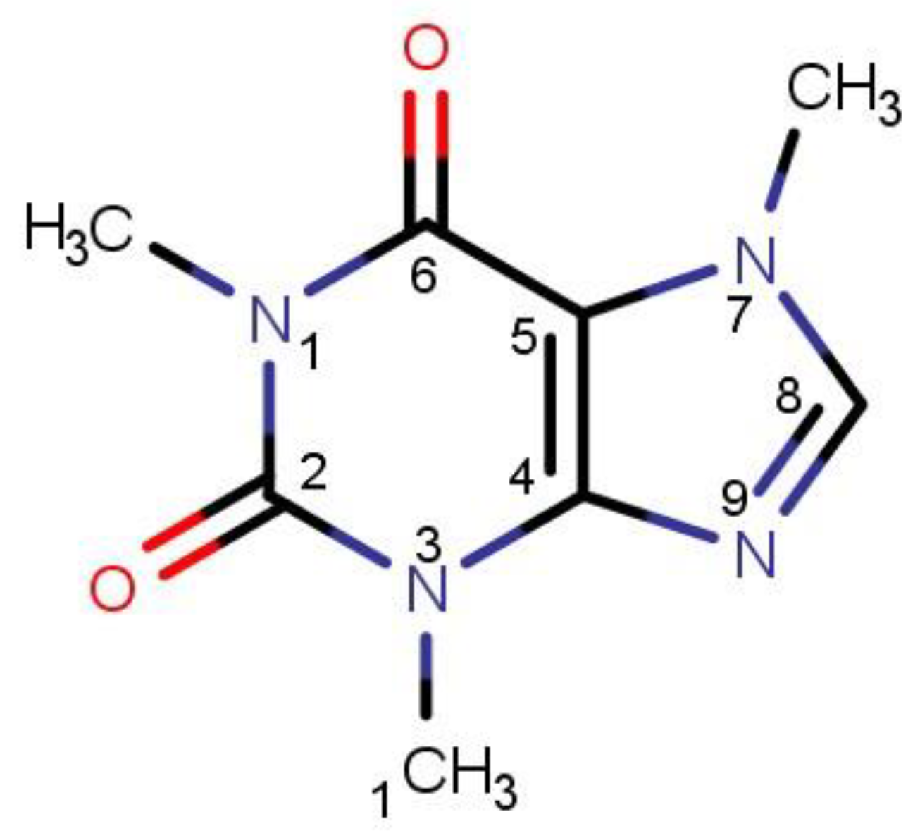
Methylxanthines, belonging to a broad range of alkaloids, are an interesting group of compounds experiencing pregnant pharmacological activity. From the perspective of the pharmaceutical manufacture, there are iii most important compounds in this category, namely theophylline (one,3-dimethylxanthine) [1], theobromine (3,seven-dimethylxanthine) [2] and caffeine (1,three,7-trimethylxanthine). Methylxanthines are arable in nature residing in tea and other plant leaves, coffee and cocoa beans, also equally cola seeds [three]. From a chemical perspective, methylxanthines are alkaloids based on purine, which is a fused heterocyclic organisation containing both pyrimidine and imidazole rings [4]. Methylxanthines are more often than not fairly poorly soluble in h2o and ethanol [5] and have a low water–octanol sectionalisation coefficient [six]. While theophylline and theobromine are amphiprotic compounds, caffeine does not possess acidic properties [7] due to the methylation of all heteroatoms. Methylxanthines are readily captivated in the gastrointestinal tract and tin can penetrate to the central nervous arrangement where their psychostimulating properties are visible. The activities of methylxanthines include stimulation of the central nervous system, increase of blood force per unit area, diuresis of kidneys, relaxation of smooth muscles, strengthening of the concentration of skeletal muscles or gastric acrid secretion [eight,9]. These activities are the result of the power of methylxanthines to act every bit phosphodiesterase inhibitors [10] and nonselective adenosine receptor antagonists [11]. Caffeine (structural formula presented in Figure ane), one of the 3 most pharmacologically important methylxanthines as mentioned before, is plant in many plants traditionally associated with the presence of methylxanthines [12,xiii]. It has been consumed by humans for thousands of years with the primeval accounts dating back to aboriginal Communist china [14,15], from which the custom of using this compound in the form of brewed tea and java would spread effectually the world, although caffeine was isolated for the start time in 1819 and synthesized in 1865 [16]. Nowadays it is estimated that about 80% of the world's adult population consumes 200–250 mg of caffeine every day [17,18]. The absorption of caffeine from the small intestine after oral intake is rapid and complete [19] and its elimination from the organism occurs mainly through excretion in urine with paraxanthine being the main metabolite [twenty]. The mode of activity of caffeine is related to binding to adenosine receptors [21] and inducing psychomotor stimulant properties in the brain [19]. The beneficial effects of caffeine comprise improved alacrity, mood and performance, reduced fatigue and alleviated effects of slumber impecuniousness [22,23,24], although its excessive consumption can atomic number 82 to several side effects [21,25,26].

The solubility of unlike active pharmaceutical ingredients (APIs) is a crucial parameter utilized in the pharmaceutical industry and their inadequate solubility is a well-recognized limitation [27] in the development of new drugs. For example, according to BCS (Biopharmaceutics Nomenclature System) criteria, as many every bit 40% of drugs can be regarded as practically insoluble in water [28] and this number is even higher for newly developed drugs [29]. There are many strategies used to overcome this difficulty including amorphization [30,31], formation of monocrystals [32,33], micronization [34] and solid dispersion formation [35], complexation with cyclodextrins [36,37], salts [38,39] and cocrystals formation [40,41]. Using cosolvation techniques is another fashion of increasing solubility. The cosolvation effect takes place when a particular amount of a cosolvent is added to the primary solvent and causes a solubility increment [42,43]. Different organic compounds can be used for this job, including DMSO, ethylene glycol, propylene glycol, glycerin, ethanol and others [44]. Studies evidence that the usage of cosolvents may lead to a solubility increment of fifty-fifty several hundred times [45]. The machinery of solubility comeback due to cosolvation is all the same extensively studied. More often than not speaking, cosolvency increases the solubility of hydrophobic/lipophilic drugs by disturbing the intermolecular network of hydrogen bonds nowadays in aqueous systems. This in turn lowers the polarity of the system and creates an environment with physicochemical properties closer to those of the drug, according to the full general rule that "similar dissolves in a similar" [46]. Very of import in the context of the applied application of cosolvation techniques are the considerations regarding the design of cosolvent systems and their influence on drug solubility [44,47,48,49] often combined with other strategies addressing low drug solubilization. These tin include the pH modification of the solution [50], the utilise of surfactants [51,52] or complexation with cyclodextrins [53,54].

Caffeine solubility was extensively studied experimentally in neat organic solvents [55,56,57], binary solvent mixtures [58,59,60,61,62,63,64,65,66,67] and carbon dioxide [68,69]. It is interesting to notation that in several binary solvents a cosolvency outcome was observed. For example, mixtures of methanol + carbon tetrachloride [60] and ethyl acetate + ethanol [61] offer a pregnant cosolvency effect. Furthermore, aqueous mixtures of methanol [62], ethanol [61], dimethyl formamide [60] or 1,four-dioxane [63] showroom similar behavior. To the contrary, such a phenomenon is non observed for systems comprising carbitol + ethanol [64] and Northward-methyl-ii-pyrrolidone in mixtures with ethanol [58], n-propanol [65], isopropanol [66], ethylene glycol [59] or propylene glycol [67].

Apart from traditional organic solvents, ionic liquids and deep eutectic solvents are gaining increasing attention and utilization in the context of dissolution and extraction of active pharmaceutical ingredients [70,71]. This is due to their beneficial properties including excellent solubilizing potential, ecology friendliness and relatively depression cost of preparation. Additionally, the beliefs of caffeine in these designed solvents was studied [72,73,74,75,76]. Particularly interesting are the results of caffeine extraction from spent coffee grounds using cholinium-based ionic liquids [72]. Our research team has previously published the results of theophylline and theobromine solubilized in natural deep eutectic solvents utilizing choline chloride [1,2] and similar results regarding caffeine volition follow.

The aim of this newspaper is fourfold. First of all, the total pool of caffeine experimental solubility data is extended past including aprotic proton acceptor solvents (APAS), which were used in binary mixtures with water. Secondly, the observed solubility trends are interpreted in terms of intermolecular interactions quantified using an avant-garde level of quantum chemistry computations. Thirdly, the gathered information is used for screening with the purpose of finding more environmentally friendly and constructive solvents. Finally, the hypothesis formulated at the screening phase is validated past additional solubility measurements aimed at increasing the ecology safety of caffeine dissolution.

2. Materials and Methods

2.ane. Materials

The main compound used in this study was caffeine (CAS: 58-08-2, MW = 194.19 m/mol) purchased from Sigma Aldrich, Saint Louis, MO, U.s., with a purity of ≥99%. All of the utilized organic solvents were supplied by Avantor Functioning Materials, Gliwice, Poland. These were the following: methanol (CAS: 67-56-1), dimethyl sulfoxide-DMSO (CAS: 67-68-5), dimethylformamide-DMF (CAS: 68-12-2), i,4-dioxane (CAS: 123-91-i), acetonitrile (CAS: 75-05-viii), acetone (CAS 67-64-1) and 4-formylmorpholine (CAS: 4394-85-8). All solvents had a purity of ≥99% and were used without any initial procedures.

2.two. Preparation of the Calibration Curve

In order to obtain a calibration curve for caffeine, its stock solution was prepared with a concentration equal to 3.23 mg/mL in a 100 mL volumetric flask using methanol as a solvent. And so, successive dilutions were made by transferring specific volumes of the stock solution into x mL volumetric flasks and diluting them with methanol, thus obtaining a series of caffeine solutions with decreasing concentration. Spectrophotometric measurements of such solutions were conducted and the values of absorbance at 272 nm wavelength were plotted against the concentration values. 3 separate series of measurements were performed and the final curve resulted from averaging. The statistical analysis of the obtained curve included the determination coefficient R², limit of detection (LOD) and limit of quantification (LOQ). Details regarding the scale curve can exist found in Supplementary Materials in Tabular array S1a,b.

two.3. Training of Samples in Aqueous Binary Mixtures of Organic Solvents

For preparing the solvent mixtures utilized in the report, preset amounts of the organic solvent and h2o were mixed together in 10 mL volumetric flasks with different mole ratios. Next, excess amounts of caffeine were placed in exam tubes which were then filled with the solvent mixture prepared earlier or with a neat solvent. This way saturated solutions of caffeine were obtained. The prepared samples were incubated for 24 h at different temperatures using an Orbital Shaker Incubator ES-twenty/60 supplied by Biosan, Riga, Latvia. The temperature aligning accurateness was 0.i °C and its variance during the daily cycle was ±0.v °C. The mixing of the samples at lx rev/min was provided by the incubator. Afterwards incubation, the samples were filtered with the assist of a syringe equipped with a PTFE filter with 22 µm pore size. All of the test tubes, syringes and filters were preheated at the appropriate temperature to avoid atmospheric precipitation of dissolved caffeine. Next, fixed amounts of the filtrate were transferred to test tubes filled with a fix amount of methanol and the diluted samples were measured spectrophotometrically. In lodge to establish the mole fractions of caffeine in solutions, the density of the samples was determined.

2.4. Solubility Measurements

The caffeine concentration in the samples was measured spectrophotometrically with the utilise of an A360 spectrophotometer from AOE Instruments, Shanghai, People's republic of china. The procedure involved obtaining spectra in the 190–700 nm wavelength range with a 1 nm resolution and utilizing the absorbance values at 272 nm. Since methanol was used for diluting the samples it was as well used as a reference during spectrophotometric measurements. Furthermore, in guild for the absorbance to remain in the linearity limit of the calibration curve, the samples were diluted accordingly using methanol. Three samples were measured for each arrangement and their concentrations were averaged and expressed equally mole fractions.

2.5. FTIR–ATR Measurements

Solid sediments of caffeine were analyzed by FTIR-ATR measurements subsequently collecting residues from the test tubes after solubility experiments described above. The samples were dried and measured using an FTIR Spectrum 2 spectrophotometer from Perkin Elmer, Waltham, MA, USA, equipped with a diamond adulterate total reflection (ATR) device. The spectra were recorded in the 450–4000 cm⁻¹ wavenumber range.

two.6. Differential Scanning Calorimetry Measurements

The characterization of caffeine beliefs in the presence of h2o, organic solvents and their mixtures was conducted using the differential scanning calorimetry (DSC) technique. Firstly, 0.4 g of caffeine samples were basis with appropriate amounts of unlike solvents using a MM 200 manufactory from Retsch, Haan, Germany. The frequency was set to 25 Hz and the grinding lasted for 30 min. Jars (5 mL) from stainless tell were used for grinding the samples with 2 stainless steel balls. For calorimetric measurements, the DSC 6000 from PerkinElmer, Waltham, MA, Usa, was used with a heating charge per unit of 10 K/min and twenty mL/min nitrogen flow for providing an inert temper. Standard aluminum pans were used for the measurements and the calorimeter was initially calibrated with indium and zinc standards.

2.7. Affinity Breakthrough Chemistry Computations

Although solubility tin be sometimes explained in terms of solvation energy [77], we can offer a much meliorate relationship betwixt computed values of Gibbs free energies and experimental solubility, even though information technology seems that such trend is of local grapheme and holds for a given compound or a class of compounds in a limited range of solvents. Therefore, in this work, we take interpreted the solubility of caffeine in terms of solute–solvent intermolecular interactions.

Intermolecular interactions of caffeine were modeled using an advanced breakthrough chemical science level including electron correlation corrections and nothing-point vibrational energy ZPE. The computational protocol follows an already presented methodology [2,78,79,eighty,81] and here just a cursory summary is provided. It is causeless that the solute–solvent affinity between constituents of considered binary solvents tin can be expressed, as the first approximation, in terms of corresponding reactions of pair formation, namely X + Y = XY, where X and Y stand either for solute or solvent molecules. In the example of 10 = Y dimers are formed of AA, BB1 or BB2 type, where A stands for caffeine, B1 for organic solvent and B2 represents a water molecule. The other three hetero-molecular complexes, namely AB1, AB2 and BB12, consummate the variations of all possible binary contacts. The applied calculations of the thermodynamic properties require a reasonable representation of the molecular structure both in the gas and in the condensed phases. Since many molecules can exist in a variety of conformers, which can impact the structure of bimolecular contacts, extensive conformational screening of biomolecular systems was performed. Many potential bimolecular clusters were considered by automatic generation of structures with the highest probability of interactions between the surface segments of molecules, which is offered by the COSMOtherm program [82] via invoking the control "CONTACT = {1 two} ssc_probability ssc_weak ssc_ang = fifteen.0". This typically leads to a quite big number of potential structures, which further undergo geometry optimization and clustering. The optimization of structures was carried out using RI-DFT BP86 (B88-VWN-P86) with def-TZVP basis set, which was followed past single-point energy computations using def2-TZVPD basis gear up with the fine grid tetrahedron cavity and inclusion of parameter sets with hydrogen bond interaction and van der Waals dispersion term based on the "D3" method of Grimme et al. [83]. All quantum chemistry calculations were performed using TURBOMOLE version 7.v.one [84] interfaced with BIOVIA TmoleX version 21.0.1. [85]. The values of Gibbs complimentary energies were determined using COSMOtherm version 21.0.0 [82] with BP_TZVPD_FINE_21.ctd parametrization.

Computations of the equilibrium constant are realized in COSMOtherm via a typical thermodynamic cycle scheme. It involves geometry optimization both in the gas and bulk phases followed by thermal free energy contribution determined via the COSMO-RS arroyo, equally summarized in Scheme 1. The thermodynamic characteristics of the reaction in the gas phase is the first footstep, which critically determines the accurateness of predicted values of equilibrium constant. Information technology is essential to emphasize that currently COSMOtherm parameterizations are restricted to density functional theory (DFT) models, which make up one's mind the accurateness of the reaction energy. In particular, the BP86 functional is used in the bulk of concrete properties computations. Due to its inherent limitations, it is necessary to go across DFT using loftier-level quantum chemical science computations for enhancing the accuracies of energy determination. Hence, three types of corrections to the values of electronic energy are added for accurate computations of the full gas phase energy, namely (1) accounting for the electron correlation energy,

$\Delta {\mathrm{Eastward}}_g^{cor}$

, improperly computed using merely the DFT level, (2) correction for the zilch Kelvin vibrational energy,

$\Delta {\mathrm{Eastward}}_g^{ZPE}$

, and (3) basis superposition error. Since the gas stage properties can be significantly affected by the accurateness of computations [86], the electron correlation computed on RI-MP2 level of theory was included using an extended Ahlrichs def2-QZVPP ground set [87] utilizing the geometry determined in the previous pace, namely RI-DFT BP86/def-TZVP. Also, the values of the zilch-point vibrational energy (ZPE) were computed at RI-DFT BP86 (B88-VWN-P86)/def2-TZVPD level. The BSSE can be estimated using a DFT-C approach, which formulation includes atom–atom many-body corrections and is a parameterized geometry-based method [88]. These computations are to be performed for every conformer for all reagents and averaged with weights corresponding to population percentage estimated using Boltzmann probability. The final values of the reaction Gibbs free energy, Δ1000_r , business relationship for all thermal complimentary energy of the gas stage contribution and the Gibbs complimentary free energy of solvation quantifying the contribution of transfer from gas to liquid.

Finally, it is worth calculation that in COSMOtherm it is possible to split the contribution to the equilibrium constant into the concentration-dependent contribution, Yard₁₀ , and activeness constant, 1000_γ , bookkeeping for nonideality. The production of these constants leads to activity and therefore concentration-independent constant, K_a . Hence, for computation of this quantity, the knowledge of the actual concentration of reagents is non necessary. Practically it tin be achieved by invoking the command "K_activity" in COSMOtherm computations.

3. Results and Give-and-take

three.one. Solid Country Characteristics

Caffeine exists in ii stable polymorphic forms (termed I and II) and a hydrate, which have been a topic of many studies [89,90,91,92,93]. Form Ii is stable at temperatures beneath 151 °C, while course I is stable at college temperatures up to the melting point of 238 °C. The hydrate on the other manus is subjected to water loss at 145 °C. Additionally, a third polymorphic course was obtained through sublimation [94]. In order to observe which forms are present in the solid state obtained subsequently the solubility measurements, both DSC and FTIR techniques were used, as described in the methodology department. Although extensive studies have been performed, here only a choice of results was presented in order to provide a general perspective on the caffeine polymorphic forms nowadays in the samples.

The FTIR measurements have shown that caffeine exists in an anhydrous form in neat solvents, while the improver of water results in obtaining a hydrate. This is exemplified in the case of caffeine dissolved in h2o–DMSO mixtures, as shown in Effigy S1 in Supplementary Materials. The presented IR spectra include pure caffeine, too as the precipitates obtained after solubility experiments involving water, nifty solvent and their mixtures. Pure caffeine and the solid residue obtained later on dissolution in neat DMSO (10 = one.0) are basically identical. The feature absorption bands of this form involve C-H (alkyl) at effectually 2900 cm⁻¹, C=O at around 1650 and 1710 cm⁻ⁱ, C=C at effectually 1550 cm⁻¹ and C-N at around 1250 cm⁻¹. However, when caffeine was dissolved in water and in mixtures containing water (x = 0.2 to ten = 0.8) an additional new wide band appears with a maximum at effectually 3400 cm⁻¹, which tin be attributed to the O-H stretching in the hydrate [95]. The in a higher place pattern was repeatedly observed for all studied solvents.

When taking into account the DSC measurements of the studied samples, a similar picture emerges as it was in the case of FTIR studies. Again, for practical purposes, the results obtained for DMSO–h2o mixtures are presented in Figure S2 in Supplementary Materials. The melting signal of pure caffeine, equally well as the precipitates, was establish in all cases at around 238 °C, with a mean value of 238.32 °C (standard divergence, SD = 0.39 °C) for the whole dataset, which is in skillful accordance with literature data. Nonetheless, there are differences in the position of the beginning endothermic height between the samples. In the case of pure caffeine and the sample obtained later dissolution in bang-up solvents a peak with a mean value of 157.87 °C (SD = 0.38 °C) can exist observed, which tin be attributed to the transition between forms II and I, although information technology is shifted towards higher temperatures. For the samples obtained after caffeine solubilization in mixtures containing water, a summit with a maximum of 151.66 °C (SD = 0.55 °C) was found, which again is slightly shifted compared with literature but can be assigned to the h2o loss of the caffeine hydrate. All the above observations betoken that the presence of h2o in the solvent mixtures results in the presence of the caffeine hydrate, while the lack of water is responsible for the presence of its polymorphic form II.

three.2. Experimental Solubility of Caffeine

Earlier the bodily solubility experiments, in guild to confirm the reliability and capability of the used methodology, some of the results were compared with literature data. When analyzing these results it became evident that in that location are some discrepancies in the data provided by unlike authors. However, the results obtained in this study are quite close to the ones obtained by Shalmashi et al. [56] and Dabir et al. [57] with slightly larger differences when compared with Zhong et al. [55]. Detailed results of this comparison tin can be found in Tabular array S2 in Supplementary Materials, where the mole fractions of caffeine in various solvents at dissimilar temperatures were presented together with relative differences between datasets. This analysis, supported by the fact that the results obtained for the two other methylxanthines [1,2] match literature data, suggest the adequacy of the method used in the written report.

The 5 mentioned organic solvents were used to create binary solvents with h2o in different mole proportions. For each solvent–h2o system, twelve unlike compositions were studied including both groovy solvent and water. The temperature range was set from 25 °C to 40 °C with 5 °C intervals. For all of the studied solvents, the increasing temperature resulted in an increase of caffeine solubility and the general trend of solubility profiles remains the aforementioned in all cases. The obtained results are collected in Figure 2 and the corresponding detailed values of caffeine mole fractions can be establish in Supplementary Materials, Tables S3–S7.

When using DMSO every bit a cosolvent with water a gradual increase in solubility is observed up to the point corresponding to unimolar proportions of water and DMSO (10₂ ^* = 0.5) with a less pronounced decrease subsequently. The highest value of caffeine solubility at this indicate was equal to x_C = (425.89 ± 0.92)∙10^−iv at 40 °C which is 65% more than for the cracking organic solvent.

The tendency of solubility changes observed for DMF is rather like to that of the former solvent. Again, after an increase in caffeine solubility, an inflection point can be observed at 10_two ^* = 0.5 with the highest mole fraction equal 10_C = (383.96 ± 2.16)∙10^−iv at twoscore °C, which stands for a 90% increase in solubility compared to great DMF. In both of the above solvents, the solubility decline after reaching the point of the optimal limerick is less pronounced than the initial increase of solubility.

When taking into account 1,4-dioxane as a cosolvent, somewhat similar beliefs of the caffeine solubility profile is observed. Again the unimolar proportions of h2o and the organic solvent are responsible for the largest solubility of caffeine. In this case the mole fraction obtained at 40 °C for 10₂ ^* = 0.5 was 10_C = (269.77 ± 2.59)∙10⁻⁴. Contrary to DMSO and DMF however, the subsequently decrease of caffeine solubility is much more axiomatic as the highest solubility value is more than than iii times larger than the solubility obtained for pure 1,4-dioxane.

Furthermore, in the instance of acetone, the highest solubility of caffeine was observed when the proportions of water and the organic solvent were equal to each other. Hither, the highest solubility found at 40 °C equaled 10_C = (186.51 ± 0.95)∙10⁻⁴, which stood for a more than than ii times increase in solubility when compared to groovy acetone. Interestingly and contrary to the three former solvents, the composition of x₂ ^* = 0.32 was also responsible for quite loftier values of caffeine solubility, larger than the ones obtained at x_ii ^* = 0.68. Therefore, the interval of particularly elevated solubility values of caffeine was also wider than in the one-time cases.

While the overall trend of caffeine solubility changes for acetonitrile is rather similar to the one observed for acetone, at that place is one interesting feature of the obtained results. The highest solubility constitute for x₂ = 0.5 at xl °C was equal to 10_C = (202.forty ± ane.88)∙10⁻⁴ which is college than for acetone. This means that although pure acetonitrile experiences lower caffeine solubility than pure acetone, the binary mixture of acetonitrile and water is more efficient than the corresponding binary solvent involving acetone. Furthermore, the solubility obtained at the point of the optimal composition is more than 4 times college than the one obtained for the neat solvent, which is the highest among studied solvents.

3.3. Caffeine Interactions in Studied Solvents

Observed solubility trends can exist interpreted in terms of intermolecular interactions. For this purpose, the affinities of caffeine toward hetero-molecular pairs formation were calculated using quantum chemistry computations on an advanced level, equally described in the methodology department. Selected structural and energetic properties are collected in Tabular array ane.

Quite surprising conclusions tin be drawn from the results provided in Table 1, namely, caffeine can act as a donor in pairs formation with all considered APAS. The hydrogen cantlet bound to the carbon atom within the five-membered ring (C₈) has quite an acidic character and can be straight involved in non-covalent interactions with solvent molecules. Hence, negative centers located on oxygen atoms of solvent molecules can complete the pair formation with proton-accepting sites. On the contrary, with proton donating molecules, for case, water, caffeine plays the role of an acceptor in pair germination via the basic center of the nitrogen atom (N_nine) located on the imidazole ring. The same feature might be observed for alcohols and other proton donating molecules. In the case of caffeine contacts with aprotic solvents, molecules of the formed pairs can be considered as examples of weak hydrogen bonds. This tin be interfered with past geometric features of the considered pairs. Information technology is evident that hydrogen bonds are much longer in all cases of apolar solvents if compared with the caffeine–water hydrogen-bonded pair. Despite this fact, the stabilization of pairs of DMF and DMSO with caffeine is as loftier every bit in the water complex. This is in interesting correspondence with the loftier solubility of caffeine in these solvents. The interactions of caffeine with the other three apolar solvents are weaker, with the smallest stabilization of pairs formed with acetonitrile, and this social club as well corresponds to the observed solubility. It is also worth highlighting that the interest of the C_viii cantlet of caffeine might be anticipated after inspection of the electrostatic potential distribution. This is documented in Figure 3 by plotting the isosurface in the range of <−0.05 eV, +0.05 eV>. It is conspicuously visible that at that place is a very large blueish region in the vicinity of the hydrogen atom involved in pairs formation with aprotic molecules, indicating an electropositive character of this fragment of caffeine. Hence, this ascertainment might be used in anticipating interactions with apolar solvents with negative centers.

3.iv. Solubility Estimation in Terms of Caffeine Intermolecular Interactions

Previously mentioned qualitative agreement between the computed solute–solvent affinities and measured solubility of caffeine is the starting point for further exploration of the usefulness of the computed values of caffeine affinities as a potential prognostics of its solubility. For this purpose, plots were prepared relating the experimental solubility with computed values of Gibbs free energies of self- and hetero-clan of solute–solute (AA), solute–solvent (AB) and solvent–solvent (BB) interactions. The former includes merely caffeine dimerization. The 2d blazon comprises two kinds of contributions coming from interactions with water and the organic solvent. The latter type involves all homo- and hetero-pairs formed between solvent molecules. The obtained results are provided in Figure 4. In item, AA denotes caffeine dimerization, AB1 caffeine-organic solvent pairs formation, AB2 caffeine-water pairs germination, BB1 organics self-association, BB2 water dimerization and BB12 hetero-association of solvent molecules.

The results provided in Figure 4 reveal a quantitative human relationship between caffeine affinities and the measured solubility values. It is worth mentioning that values of ΔOne thousand_r used for plots preparation correspond to concentration-dependent equilibrium constants (K_x ) rather than the activity ones (1000_a ), which were included in Table 1. By separating mole fraction contributions to equilibrium constants from contributions coming from the activity coefficient it is also possible to inspect how the concentration of the solvent affects the affinity ΔThousand_r ^(x) , as seen in Figure 5. It seems that at that place is a correlation between experimental solubility and solute–solvent affinities with acceptable linearity (R² = 0.78) of this relationship. Hence, Figure 4 further documents the importance of direct contacts of caffeine, although the beingness of linear relationships is not and then obvious taking into account that only pairs are included in the solubility modeling. Caffeine dimerization, although much less favorable nether all studied conditions, also exhibits a linear relationship with respect to experimental solubility. However, total intermolecular interaction including all possible contacts is a much less reliable prognostic for solubility predictions. Probably including many potential multi-molecular complexes in the model would exist benign. Unfortunately, this is prevented non only by the number of potential structures to be considered but also by the expense of computations, which include not merely zero-point energy correction just besides cover electron correlation and dispersion corrections.

three.5. Screening of Caffeine Solubility

The observation of a semi-quantitative linear correlation of caffeine solubility in systems comprising apolar solvents with computed solute–solvent affinities offers the possibility of screening for new solvents belonging to the aforementioned class. The set of organic solvents used in this paper consists of commonly used ones. Although their backdrop are well recognized, some of their features are often ignored, such as, for example, ecology impact. The nigh spectacular example is DMSO. It is generally considered a greenish, safety and non-toxic solvent. However, according to classification by the U.S. Ecology Protection Bureau (EPA) [96], the overall environmental index (EI) is every bit loftier every bit 11.68. This index is defined as a sum of many contributions including scores characterizing Human Toxicity Potential past Ingestion, past Inhalation, Terrestrial Toxicity Potential, Aquatic Toxicity Potential, Global Warming Potential, Ozone Depletion Potential, Photochemical Oxidation Potential (PCOP) and Acid Rain Potential [97]. In the case of DMSO, the source of such a high value of EI originates from the very high PCOP contribution. This parameter quantifies the stability of a given compound by comparing the charge per unit of a chemical reaction with a hydroxyl radical to the rate of an analogical reaction of ethylene. In the instance of DMSO, this parameter has a dominant influence on the overall value of EI. After excluding this score from summation, the obtained environmental index drops downward to EI(PCOP = 0) = 0.26 suggesting the greenness of DMSO. However, with DMSO and DMF, there are several associated warnings such as potential source of skin irritation, serious eye irritation, possible respiratory irritation and as well specific toxicity for many organs. Acetone, acetonitrile and 1,4-dioxane, autonomously from these warnings, are also flammable and harmful if swallowed. Hence, information technology is of crucial importance to as well include the potential environmental impact in the solubility analysis and such information regarding these common solvents is provided in Tabular array 2. Nowadays [eighty], screening for the well-nigh efficient and, at the same time, light-green solvents for sulfamethizol turned our attention toward morpholine analogs, among which many can be considered as APAS. A curt listing of such potential solvents is also provided in Tabular array 2. The listing was restricted only to such solvents which are aprotic and greener when compared to common solvents. It is worth noting that 4-formylmorpholine (4FM) is characterized by the smallest value of EI and seems to exist the first selection alternative to studied solvents. Taking reward of the linear relationship between solubility and solute–solvent affinities information technology is possible to predict solubility in new solvents. Even though only a small linear relationship is observed, the qualitative agreement allows for narrowing the list of solvents potentially interesting for experimental solubility conclusion. The results of analogousness computations for selected morpholines are collected in Table 3. Information technology is straight visible that the structural motif of solute–solvent contacts formation resembles the ones previously observed for other APAS. Both the geometrical parameters of hydrogen bonding and the energetics of pair germination with caffeine advise that all morpholines tin can human activity equally effective solvents. Interestingly, the affinities of methyl and ethyl analogues are slightly higher compared to 4FM and morpholine. Every bit information technology was evidenced in Table 2, four-formylmorpholine is the near interesting solvent due to the lowest value of EI. Hence, 4FM was selected for testing the presented above hypothesis that the affinity of solute can exist a valuable and directly guidance for selection of culling solvents. Thus, caffeine solubility in 4FM was measured for quantification of the solubilizing potential of this APAS. The results obtained at 25 °C are collected in Figure 6, with corresponding details bachelor in the Supplementary Materials, Table S8. For comparison purposes, the solubility of caffeine in DMSO is also provided in the effigy.

The full general trend of caffeine solubility in solutions comprising the selected solvent and water in varying mole compositions is analogical to the ones obtained earlier. The highest solubility, i.e., x_C = (325.52 ± four.58)∙x^−four was found for the composition with unimolar proportions of both binary solvent constituents. Using pure 4FM as the solvent resulted in the solubility of caffeine equal ten_C = (212.80 ± i.53)∙10⁻⁴. The obtained results indicate that this organic solvent is more constructive than DMSO with caffeine solubility increased by 10.3% in the optimal composition and by 17.nine% in the pure solvent. This observation confirms the usefulness of the described screening procedure in finding suitable candidates for caffeine dissolution in terms of both efficiency and environmental friendliness.

4. Conclusions

The solubility of caffeine was studied in aqueous binary mixtures of some aprotic proton acceptor solvents (APAS). The performed experiments revealed that calculation a specific amount of h2o to the studied organic solvents resulted in achieving a cosolvation result and ultimately in an increase of caffeine solubility compared to great solvents. In all cases, a unimolar amount of water and organic solvent was responsible for the largest obtained solubility of caffeine. The highest solubilization efficiency was observed for the DMSO–h2o organisation and in the optimal limerick at 40 °C the caffeine solubility was found to be x_C = (425.89 ± 0.92)∙10⁻⁴, which amounts to about 65% increase compared to neat DMSO. The order of decreasing solubilizing potential of binary systems containing water and organic solvents is as follows: DMSO > DMF > 1,4-dioxane > acetonitrile > acetone. A full general trend shows that smaller caffeine solubilities in nifty solvents are associated with a higher solubility gain in the optimal compositions.

In order to interpret the observed solubility trends, the affinities of caffeine toward hetero-molecular pairs germination were studied using advanced quantum chemistry computations. It was plant that caffeine can deed equally a donor in pairs formation with all considered APAS. This is due to the hydrogen atom jump to the carbon cantlet within the five-membered ring (C₈), which thank you to its electropositive graphic symbol tin exist involved in interactions with negative centers located on oxygen atoms of solvent molecules, which tin be considered as weak hydrogen bonds. There was institute an interesting correspondence between the stabilization of the formed pairs and the observed experimental solubility, namely the larger stabilization was associated with higher solubility of caffeine. Furthermore, the knowledge nigh the electropositive region in a solute molecule can be used to anticipate interactions with apolar solvents containing negative centers. The computed values of Gibbs free energies of self-clan and intermolecular pairs germination of solute–solute, solute–solvent and solvent–solvent interactions were further studied for exploring the possibility of using them as potential solubility prognostics. A semi-quantitative relationship between caffeine affinities and the measured solubility values was found, with the highest linearity (R² = 0.78) observed in the case of caffeine–solvent interactions.

The observed fact that caffeine solubility in systems comprising apolar solvents is correlated with computed solute–solvent affinities enables screening for new solvents of the same class. The environmental touch on of many solvents is a factor limiting their applications and therefore there is a demand for alternative ones. The environmental index (EI) offered by the U.Due south. Environmental Protection Bureau (EPA) is a measure of environmental touch used for suggesting solvents for caffeine dissolution alternative to DMSO. Based on previous experience, morpholine analogs, amongst which many can be considered as aprotic solvents, were suggested as an interesting culling. A list of potential solvents was created and, based on their EI indices, the 4-formylmorpholine was selected for solubility experiments. It turned out that this solvent was even more effective in caffeine dissolution than DMSO both in the neat form, as well as in a binary mixture in unimolar proportions with h2o. The obtained effect shows the usefulness of such types of screening in the search for environmentally-friendly replacements of traditional solvents.

Supplementary Materials

The following supporting information can be downloaded at: https://world wide web.mdpi.com/article/ten.3390/ma15072472/s1, Figure S1. The FTIR spectra of caffeine precipitates obtained afterwards solubility measurements in DMSO, water and their mixtures. Values in the legend signal the mole fractions of DMSO in solute-free binary solvents. For comparing, the spectrum of pure caffeine is shown. Figure S2. The DSC curves of caffeine precipitates obtained after solubility measurements in DMSO, water and their mixtures. Values in the figure indicate the mole fractions of DMSO in solute-free binary solvents. For guiding the eye vertical lines are drawn corresponding to the hydrate h2o loss (dashed line) and the transition from form II to grade I (dotted line). For comparison, the DSC curve of pure caffeine is also provided. Table S1a. Concentrations of caffeine solutions and the respective absorbance values, together with mean absorbance and standard difference (SD) values, used during preparation of the calibration curve. Table S1b. Parameters of the obtained calibration curve for caffeine solubility determination. Table S2. Comparing of caffeine solubility values expressed every bit mole fractions (∙10^four) obtained in this study and the results taken from literature. Standard deviation values (∙10^four) are given in parentheses. Relative differences betwixt datasets are also provided. Table S3. Mole fractions (∙10⁴) and standard deviation (SD) values (∙ten^iv) of caffeine in binary solvents comprising water and DMSO in unlike proportions. Table S4. Mole fractions (∙10^four) and standard deviation (SD) values (∙10⁴) of caffeine in binary solvents comprising water and DMF in different proportions. Table S5. Mole fractions (∙x^iv) and standard deviation (SD) values (∙10^iv) of caffeine in binary solvents comprising water and dioxane in unlike proportions. Table S6. Mole fractions (∙10^four) and standard deviation (SD) values (∙10^iv) of caffeine in binary solvents comprising water and acetone in unlike proportions. Table S7. Mole fractions (∙10⁴) and standard deviation (SD) values (∙10^four) of caffeine in binary solvents comprising water and acetonitrile in different proportions. Tabular array S8. Mole fractions (∙ten⁴) and standard deviation (SD) values (∙10^four) of caffeine in binary solvents comprising water and 4-formylmorpholine in dissimilar proportions at 25 °C.

Writer Contributions

Conceptualization, P.C. and T.J.; Methodology, P.C. and T.J.; Software, P.C.; Validation, T.J. and M.Thousand.; Formal Analysis, P.C.; Investigation, T.J., P.C. and M.K.; Resources, P.C.; Data Curation, T.J., M.K. and P.C.; Writing—Original Typhoon Grooming, P.C. and T.J.; Writing–Review and Editing, T.J. and P.C.; Visualization, P.C.; Supervision, P.C.; Projection Administration, T.J.; Funding Acquisition, P.C. All authors accept read and agreed to the published version of the manuscript.

Funding

This research received no external funding.

Institutional Review Lath Statement

Non applicable.

Informed Consent Statement

Not applicable.

Data Availability Statement

Not applicative.

Conflicts of Interest

The authors declare no conflict of interest.

References

1. Cysewski, P.; Jeliński, T.; Cymerman, P.; Przybyłek, M. Solvent screening for solubility enhancement of theophylline in cracking, binary and ternary NADES solvents: New measurements and ensemble machine learning. Int. J. Mol. Sci. 2021, 22, 7347. [Google Scholar] [CrossRef] [PubMed]
2. Jeliński, T.; Stasiak, D.; Kosmalski, T.; Cysewski, P. Experimental and theoretical study on theobromine solubility enhancement in binary aqueous solutions and ternary designed solvents. Pharmaceutics 2021, 13, 1118. [Google Scholar] [CrossRef]
3. Dolder, L.K. Methylxanthines: Caffeine, Theobromine, Theophylline. In Small Beast Toxicology, 3rd ed.; Petersen, M.Eastward., Talcott, P.A., Eds.; Saunders: St. Louis, MO, USA, 2013; pp. 647–652. [Google Scholar] [CrossRef]
4. Ashihara, H.; Sano, H.; Crozier, A. Caffeine and related purine alkaloids: Biosynthesis, catabolism, part and genetic engineering science. Phytochemistry 2008, 69, 841–856. [Google Scholar] [CrossRef] [PubMed]
5. Jouyban, A. Handbook of Solubility Data for Pharmaceuticals, 1st ed.; CRC Press: Boca Raton, FL, Us, 2010. [Google Scholar] [CrossRef]
6. Hansch, C.; Leo, A.; Hoekman, D. Exploring QSAR: Volume two: Hydrophobic, Electronic, and Steric Constants, 1st ed.; American Chemical Guild: Washington, WA, The states, 1995. [Google Scholar]
7. Andreeva, Eastward.Y.; Dmitrienko, Southward.G.; Zolotov, Y.A. Methylxanthines: Properties and conclusion in various objects. Russ. Chem. Rev. 2012, 81, 397–414. [Google Scholar] [CrossRef]
8. Craig, C.R.; Stitzel, R.E. Modernistic Pharmacology with Clinical Applications, 6th ed.; Lippincott Williams and Wilkins: Philadelphia, PA, USA, 2003. [Google Scholar]
9. Satoskar, R.S.; Rege, Northward.; Bhandarkar, Southward.D. Pharmacology and Pharmacotherapeutics, 24th ed.; Elsevier Bharat: New Delhi, India, 2015. [Google Scholar]
10. Essayan, D.M. Cyclic nucleotide phosphodiesterases. J. Allergy Clin. Immunol. 2001, 108, 671–680. [Google Scholar] [CrossRef] [PubMed]
11. Müller, C.E.; Hibernate, I.; Daly, J.Westward.; Rothenhausler, K.; Eger, K. vii-Deaza-two-phenyladenines: Structure-action relationships of potent A1 selective adenosine receptor antagonists. J. Med. Chem. 1990, 33, 2822–2828. [Google Scholar] [CrossRef] [PubMed]
12. Frary, C.D.; Johnson, R.K.; Wang, M.Q. Food sources and intakes of caffeine in the diets of persons in the United States. J. Am. Nutrition. Assoc. 2005, 105, 110–113. [Google Scholar] [CrossRef]
13. Heckman, K.A.; Weil, J.; de Mejia, E.G. Caffeine (1, 3, vii-trimethylxanthine) in foods: A comprehensive review on consumption, functionality, safe, and regulatory matters. J. Nutrient Sci. 2010, 75, R77–R87. [Google Scholar] [CrossRef] [PubMed]
14. Fredholm, B.B. Notes on the history of caffeine apply. Handb. Exp. Pharmacol. 2011, 200, one–ix. [Google Scholar] [CrossRef]
15. Lu, H.; Zhang, J.; Yang, Y.; Yang, 10.; Xu, B.; Yang, W.; Tong, T.; Jin, Due south.; Shen, C.; Rao, H.; et al. Primeval tea as evidence for one branch of the Silk Road across the Tibetan Plateau. Sci. Rep. 2016, 6, 18955. [Google Scholar] [CrossRef] [PubMed]
16. Waldvogel, S.R. Caffeine—A drug with a surprise. Angew. Chem. Int. Ed. Engl. 2003, 42, 604–605. [Google Scholar] [CrossRef]
17. Barone, J.J.; Roberts, H.R. Caffeine consumption. Nutrient Chem. Toxicol. 1996, 34, 119–129. [Google Scholar] [CrossRef]
18. Patat, A.; Rosenzweig, P.; Enslen, M.; Trocherie, Due south.; Miget, N.; Bozon, M.C.; Allain, H.; Gandon, J.M. Effects of a new wearisome release formulation of caffeine on EEG, psychomotor and cognitive functions in sleep-deprived subjects. Hum. Psychopharmacol. 2000, 15, 153–170. [Google Scholar] [CrossRef]
19. Fisone, G.; Borgkvist, A.; Usiello, A. Caffeine every bit a psychomotor stimulant: Mechanism of action. Prison cell. Mol. Life Sci. 2004, 61, 857–872. [Google Scholar] [CrossRef] [PubMed]
20. Faber, 1000.S.; Jetter, A.; Fuhr, U. Assessment of CYP1A2 activity in clinical practice: Why, how, and when? Basic Clin. Pharmacol. Toxicol. 2005, 97, 125–134. [Google Scholar] [CrossRef]
21. Nawrot, P.; Jordan, S.; Eastwood, J.; Rotstein, J.; Hugenholtz, A.; Feeley, M. Effects of caffeine on human wellness. Nutrient Addit. Contam. 2003, twenty, 1–30. [Google Scholar] [CrossRef] [PubMed]
22. Del Coso, J.; Salinero, J.J.; Lara, B. Effects of caffeine and coffee on man operation. Nutrients 2020, 12, 125. [Google Scholar] [CrossRef] [PubMed]
23. AlAmmar, W.A.; Albeesh, F.H.; Khattab, R.Y. Nutrient and mood: The corresponsive upshot. Curr. Nutr. Rep. 2020, 9, 296–308. [Google Scholar] [CrossRef]
24. Drake, C.; Roehrs, T.; Shambroom, J.; Roth, T. Caffeine effects on sleep taken 0, 3, or 6 hours before going to bed. J. Clin. Slumber Med. 2013, ix, 1195–1200. [Google Scholar] [CrossRef] [PubMed]
25. Lagarde, D.; Batejat, D.; Sicard, B.; Trocherie, Due south.; Chassard, D.; Enslen, M.; Chauffard, F. Wearisome-release caffeine: A new response to the effects of a limited sleep deprivation. Sleep 2000, 23, 651–661. [Google Scholar] [CrossRef] [PubMed]
26. Temple, J.L.; Bernard, C.; Lipshultz, S.Eastward.; Czachor, J.D.; Westphal, J.A.; Mestre, K.A. The safety of ingested caffeine: A comprehensive review. Front. Psychiatry 2017, 8, 80. [Google Scholar] [CrossRef]
27. Göke, M.; Lorenz, T.; Repanas, A.; Schneider, F.; Steiner, D.; Baumann, K.; Bunjes, H.; Dietzel, A.; Finke, J.H.; Glasmacher, B.; et al. Novel strategies for the formulation and processing of poorly h2o-soluble drugs. Eur. J. Pharm. Biopharm. 2018, 126, 40–56. [Google Scholar] [CrossRef] [PubMed]
28. Takagi, T.; Ramachandran, C.; Bermejo, M.; Yamashita, S.; Yu, L.X.; Amidon, Chiliad.Fifty. A provisional biopharmaceutical nomenclature of the superlative 200 oral drug products in the United States, Great Britain, Kingdom of spain, and Japan. Mol. Pharm. 2006, iii, 631–643. [Google Scholar] [CrossRef] [PubMed]
29. Ku, M.Due south.; Dulin, Due west. A biopharmaceutical nomenclature-based Correct-Kickoff-Fourth dimension formulation approach to reduce human being pharmacokinetic variability and project cycle time from Starting time-In-Human to clinical Proof-Of-Concept. Pharm. Dev. Technol. 2012, 17, 285–302. [Google Scholar] [CrossRef]
30. Hancock, B.C.; Parks, M. What is the true solubility reward for amorphous pharmaceuticals? Pharm. Res. 2000, 17, 397–404. [Google Scholar] [CrossRef] [PubMed]
31. Huang, Fifty.; Tong, W.-Q. Impact of solid state backdrop on developability cess of drug candidates. Adv. Drug Deliv. Rev. 2004, 56, 321–334. [Google Scholar] [CrossRef]
32. Merisko-Liversidge, E.; Liversidge, G.Chiliad. Nanosizing for oral and parenteral drug delivery: A perspective on formulating poorly-water soluble compounds using wet media milling applied science. Adv. Drug Deliv. Rev. 2011, 63, 427–440. [Google Scholar] [CrossRef] [PubMed]
33. Van Eerdenbrugh, B.; Van den Mooter, G.; Augustijns, P. Top-downward production of drug nanocrystals: Nanosuspension stabilization, miniaturization and transformation into solid products. Int. J. Pharm. 2008, 364, 64–75. [Google Scholar] [CrossRef]
34. Scholz, A.; Abrahamsson, B.; Diebold, S.M.; Kostewicz, E.; Polentarutti, B.I.; Ungell, A.-L.; Dressman, J.B. Influence of hydrodynamics and particle size on the absorption of felodipine in labradors. Pharm. Res. 2002, 19, 42–46. [Google Scholar] [CrossRef]
35. Janssens, S.; Van den Mooter, G. Review: Physical chemical science of solid dispersions. J. Pharm. Pharmacol. 2009, 61, 1571–1586. [Google Scholar] [CrossRef] [PubMed]
36. Brewster, M.E.; Loftsson, T. Cyclodextrins as pharmaceutical solubilizers. Adv. Drug Deliv. Rev. 2007, 59, 645–666. [Google Scholar] [CrossRef]
37. Rajewski, R.A.; Stella, V.J. Pharmaceutical applications of cyclodextrins. ii. in vivo drug commitment. J. Pharm. Sci. 1996, 85, 1142–1169. [Google Scholar] [CrossRef]
38. Korn, C.; Balbach, Southward. Compound choice for development—Is salt formation the ultimate answer? Experiences with an extended concept of the "100mg approach. Eur. J. Pharm. Sci. 2014, 57, 257–263. [Google Scholar] [CrossRef]
39. Serajuddin, A.T.M. Salt formation to meliorate drug solubility. Adv. Drug Deliv. Rev. 2007, 59, 603–616. [Google Scholar] [CrossRef]
40. Chadha, R.; Bhalla, Y.; Vashisht, Thou.M.; Chadha, Thou. Cocrystallization in nutraceuticals. In Recrystallization in Materials Processing, 1st ed.; Glebovsky, 5., Ed.; InTech: London, Uk, 2015. [Google Scholar] [CrossRef]
41. Vishweshwar, P.; McMahon, J.A.; Bis, J.A.; Zaworotko, Thou.J. Pharmaceutical co-crystals. J. Pharm. Sci. 2006, 95, 499–516. [Google Scholar] [CrossRef] [PubMed]
42. Smith, P.Due east.; Mazo, R.Thou. On the theory of solute solubility in mixed solvents. J. Phys. Chem. B 2008, 112, 7875–7884. [Google Scholar] [CrossRef] [PubMed]
43. Rubino, J.T. Cosolvents and Cosolvency. In Encyclopedia of Pharmaceutical Science and Applied science, 4th ed.; Swarbrick, J., Ed.; CRC Printing: Boca Raton, FL, USA, 2013; pp. 711–722. [Google Scholar] [CrossRef]
44. Jouyban, A. Review of the cosolvency models for predicting solubility of drugs in water-cosolvent mixtures. J. Pharm. Pharm. Sci. 2008, 11, 32–58. [Google Scholar] [CrossRef] [PubMed]
45. Seedher, N.; Kanojia, Thousand. Co-solvent solubilization of some poorly-soluble antidiabetic drugs. Pharm. Dev. Technol. 2009, fourteen, 185–192. [Google Scholar] [CrossRef] [PubMed]
46. Williams, H.D.; Trevaskis, North.Fifty.; Charman, S.A.; Shanker, R.M.; Charman, W.N.; Pouton, C.W.; Porter, C.J.H. Strategies to address low drug solubility in discovery and development. Pharmacol. Rev. 2013, 65, 315–499. [Google Scholar] [CrossRef]
47. Paruta, A.N.; Sciarrone, B.J.; Lordi, N.Thousand. Solubility of salicylic acid as a part of dielectric constant. J. Pharm. Sci. 1964, 53, 1349–1353. [Google Scholar] [CrossRef] [PubMed]
48. Fedors, R.F. A method for estimating both the solubility parameters and molar volumes of liquids. Polym. Eng. Sci. 1974, 14, 147–154. [Google Scholar] [CrossRef]
49. Millard, J.W.; Alvarez-Núñez, F.A.; Yalkowsky, S.H. Solubilization by cosolvents: Establishing useful constants for the log-linear model. Int. J. Pharm. 2002, 245, 153–166. [Google Scholar] [CrossRef]
50. Jain, N.; Yang, Thousand.; Tabibi, S.East.; Yalkowsky, Southward.H. Solubilization of NSC-639829. Int. J. Pharm. 2001, 225, 41–47. [Google Scholar] [CrossRef]
51. Kawakami, 1000.; Oda, N.; Miyoshi, K.; Funaki, T.; Ida, Y. Solubilization behavior of a poorly soluble drug under combined use of surfactants and cosolvents. Eur. J. Pharm. Sci. 2006, 28, vii–14. [Google Scholar] [CrossRef] [PubMed]
52. D'Errico, K.; Ciccarelli, D.; Ortona, O. Consequence of glycerol on micelle formation past ionic and nonionic surfactants at 25 degrees C. J. Colloid Interface Sci. 2005, 286, 747–754. [Google Scholar] [CrossRef]
53. He, Y.; Li, P.; Yalkowsky, S.H. Solubilization of Fluasterone in cosolvent/cyclodextrin combinations. Int. J. Pharm. 2003, 264, 25–34. [Google Scholar] [CrossRef]
54. Miyake, G.; Irie, T.; Arima, H.; Hirayama, F.; Uekama, K.; Hirano, Yard.; Okamoto, Y. Characterization of itraconazole/ii-hydroxypropyl-β-cyclodextrin inclusion complex in aqueous propylene glycol solution. Int. J. Pharm. 1999, 179, 237–245. [Google Scholar] [CrossRef]
55. Zhong, J.; Tang, N.; Asadzadeh, B.; Yan, West. Measurement and correlation of solubility of theobromine, theophylline, and caffeine in water and organic solvents at various temperatures. J. Chem. Eng. Data 2017, 62, 2570–2577. [Google Scholar] [CrossRef]
56. Shalmashi, A.; Golmohammad, F. Solubility of caffeine in water, ethyl acetate, ethanol, carbon tetrachloride, methanol, chloroform, dichloromethane, and acetone between 298 and 323 Yard. Lat. Am. Appl. Res. 2010, 40, 283–285. [Google Scholar]
57. Dabir, T.O.; Gaikar, V.M.; Jayaraman, Southward.; Mukherjee, Due south. Thermodynamic modeling studies of aqueous solubility of caffeine, gallic acid and their cocrystal in the temperature range of 303 K–363 Grand. Fluid Phase Equilib. 2018, 456, 65–76. [Google Scholar] [CrossRef]
58. Rezaei, H.; Rahimpour, E.; Ghafourian, T.; Martinez, F.; Barzegar-Jalali, Grand.; Jouyban, A. Solubility of caffeine in N-methyl-2-pyrrolidone + ethanol mixture at different temperatures. J. Mol. Liq. 2020, 300, 112354. [Google Scholar] [CrossRef]
59. Rezaei, H.; Rahimpour, E.; Martinez, F.; Zhao, H.; Jouyban, A. Study and mathematical modeling of caffeine solubility in North-methyl-2-pyrrolidone + ethylene glycol mixture at dissimilar temperatures. J. Mol. Liq. 2021, 341, 117350. [Google Scholar] [CrossRef]
60. Golubev, V.A.; Gurina, D.L. Dissolving ability of the binary solvent carbon tetrachloride—Methanol. Solubility of caffeine: Experiment, ASL model, and Doc simulation. J. Mol. Liq. 2021, 344, 117736. [Google Scholar] [CrossRef]
61. Bustamante, P.; Navarro, J.; Romero, S.; Escalera, B. Thermodynamic origin of the solubility profile of drugs showing one or two maxima against the polarity of aqueous and nonaqueous mixtures: Niflumic acid and caffeine. J. Pharm. Sci. 2002, 91, 874–883. [Google Scholar] [CrossRef] [PubMed]
62. Cárdenas, Z.J.; Jiménez, D.M.; Almanza, O.A.; Jouyban, A.; Martínez, F.; Acree, W.E. Solubility and preferential solvation of caffeine and theophylline in {methanol + h2o} mixtures at 298.fifteen K. J. Solut. Chem. 2017, 46, 1605–1624. [Google Scholar] [CrossRef]
63. Adjei, A.; Newburger, J.; Martin, A. Extended hildebrand arroyo: Solubility of caffeine in dioxane–h2o mixtures. J. Pharm. Sci. 1980, 69, 659–661. [Google Scholar] [CrossRef]
64. Rezaei, H.; Rahimpour, E.; Martinez, F.; Jouyban, A. Solubility of caffeine in carbitol + ethanol mixture at unlike temperatures. J. Mol. Liq. 2020, 301, 112465. [Google Scholar] [CrossRef]
65. Rezaei, H.; Jouyban, A.; Zhao, H.; Martinez, F.; Rahimpour, East. Solubility of caffeine in N-methyl-2-pyrrolidone + 1-propanol mixtures at unlike temperatures. J. Mol. Liq. 2022, 346, 117067. [Google Scholar] [CrossRef]
66. Rezaei, H.; Rahimpour, E.; Zhao, H.; Martinez, F.; Jouyban, A. Solubility measurement and thermodynamic modeling of caffeine in N-methyl-ii-pyrrolidone + isopropanol mixtures at unlike temperatures. J. Mol. Liq. 2021, 336, 116519. [Google Scholar] [CrossRef]
67. Rezaei, H.; Rahimpour, E.; Zhao, H.; Martinez, F.; Jouyban, A. Determination and modeling of caffeine solubility in N-methyl-2-pyrrolidone + propylene glycol mixtures. J. Mol. Liq. 2021, 343, 117613. [Google Scholar] [CrossRef]
68. Lentz, H.; Gehrig, Thousand.; Schulmeyer, J. Dynamic solubility measurements of caffeine in carbon dioxide and in carbon dioxide saturated with water. Phys. B+C 1986, 139–140, 70–72. [Google Scholar] [CrossRef]
69. Johannsen, K.; Brunner, Yard. Solubilities of the xanthines caffeine, theophylline and theobromine in supercritical carbon dioxide. Fluid Phase Equilib. 1994, 95, 215–226. [Google Scholar] [CrossRef]
70. Freire, One thousand.Chiliad.; Cláudio, A.F.Grand.; Araújo, J.G.Yard.; Coutinho, J.A.P.; Marrucho, I.M.; Canongia Lopes, J.N.; Rebelo, L.P.N. Aqueous biphasic systems: A boost brought nearly by using ionic liquids. Chem. Soc. Rev. 2012, 41, 4966–4995. [Google Scholar] [CrossRef]
71. Smith, E.L.; Abbott, A.P.; Ryder, Thousand.S. Deep Eutectic Solvents (DESs) and Their Applications. Chem. Rev. 2014, 114, 11060–11082. [Google Scholar] [CrossRef] [PubMed]
72. Ferreira, A.Thou.; Gomes, H.G.D.; Coutinho, J.A.P.; Freire, Chiliad.G. Valorization of spent java by caffeine extraction using aqueous solutions of cholinium-based ionic liquids. Sustainability 2021, thirteen, 7509. [Google Scholar] [CrossRef]
73. Cláudio, A.F.M.; Ferreira, A.M.; Freire, M.1000.; Coutinho, J.A.P. Enhanced extraction of caffeine from guaraná seeds using aqueous solutions of ionic liquids. Green Chem. 2013, 15, 2002–2010. [Google Scholar] [CrossRef]
74. Cai, C.; Li, F.; Liu, L.; Tan, Z. Deep eutectic solvents used as the greenish media for the efficient extraction of caffeine from Chinese dark tea. Sep. Purif. Technol. 2019, 227, 115723. [Google Scholar] [CrossRef]
75. Basaiahgari, A.; Priyanka, V.P.; Ijardar, Southward.P.; Gardas, R.L. Aqueous biphasic systems of amino acid-based ionic liquids: Evaluation of phase behavior and extraction capability for caffeine. Fluid Stage Equilib. 2020, 506, 112373. [Google Scholar] [CrossRef]
76. Yazdabadi, A.; Shahriari, S.; Salehifar, M. Extraction of caffeine using aqueous two-phase systems containing ionic liquid and sorbitol. Fluid Phase Equilib. 2019, 502, 112287. [Google Scholar] [CrossRef]
77. Yu, B.; Ren, H.; Piao, X. Towards adsorptive enrichment of flavonoids from honey using h-BN monolayer. Chem. Phys. Chem. 2022, 23, e202100828. [Google Scholar] [CrossRef] [PubMed]
78. Cysewski, P. Intermolecular interaction every bit a direct measure of water solubility advantage of meloxicam cocrystalized with carboxylic acids. J. Mol. Model. 2018, 24, 112. [Google Scholar] [CrossRef]
79. Cysewski, P.; Jeliński, T. Optimization, thermodynamic characteristics and solubility predictions of natural deep eutectic solvents used for sulfonamide dissolution. Int. J. Pharm. 2019, 570, 118682. [Google Scholar] [CrossRef] [PubMed]
80. Cysewski, P.; Przybyłek, M.; Rozalski, R. Experimental and theoretical screening for green solvents improving sulfamethizole solubility. Materials 2021, xiv, 5915. [Google Scholar] [CrossRef] [PubMed]
81. Cysewski, P.; Walczak, P.; Ziółkowska, D.; Grela, I.; Przybyłek, M. Experimental and theoretical studies on the Sulfamethazine-Urea and Sulfamethizole-Urea solid-liquid equilibria. J. Drug Deliv. Sci. Technol. 2021, 61, 102186. [Google Scholar] [CrossRef]
82. COSMOtherm, version 21.0.0; Dassault Systèmes; Biovia: San Diego, CA, USA, 2020.
83. Grimme, S.; Antony, J.; Ehrlich, South.; Krieg, H. A consistent and accurate ab initio parametrization of density functional dispersion correction (DFT-D) for the 94 elements H-Pu. J. Chem. Phys. 2010, 132, 154104. [Google Scholar] [CrossRef]
84. TURBOMOLE, version seven.five.1; TURBOMOLE GmbH: Frankfurt, Germany, 2020.
85. TmoleX, version 21.0.one; Dassault Systèmes; Biovia: San Diego, CA, USA, 2020.
86. Hellweg, A.; Eckert, F. Brick past brick computation of the gibbs free free energy of reaction in solution using quantum chemistry and COSMO-RS. AIChE J. 2017, 63, 3944–3954. [Google Scholar] [CrossRef]
87. Weigend, F.; Ahlrichs, R. Balanced basis sets of separate valence, triple zeta valence and quadruple zeta valence quality for H to Rn: Pattern and assessment of accuracy. Phys. Chem. Chem. Phys. 2005, 7, 3297–3305. [Google Scholar] [CrossRef]
88. Witte, J.; Neaton, J.B.; Head-Gordon, M. Effective empirical corrections for footing set superposition error in the def2-SVPD basis: gCP and DFT-C. J. Chem. Phys. 2017, 146, 234105. [Google Scholar] [CrossRef] [PubMed]
89. Waters, K.L.; Beal, G.D. Notes on the h2o content of crystalline caffeine. J. Am. Pharm. Assoc. Am. Pharm. Assoc. 1946, 35, 12–14. [Google Scholar] [CrossRef] [PubMed]
90. Bogardus, J.B. Crystalline anhydrous-hydrate stage changes of caffeine and theophylline in solvent-water mixtures. J. Pharm. Sci. 1983, 72, 837–838. [Google Scholar] [CrossRef] [PubMed]
91. Pirttimäki, J.; Laine, E. The transformation of anhydrate and hydrate forms of caffeine at 100% RH and 0% RH. Eur. J. Pharm. Sci. 1994, one, 203–208. [Google Scholar] [CrossRef]
92. Edwards, H.G.M.; Lawson, E.; Matas, Thousand.d.; Shields, L.; York, P. Metamorphosis of caffeine hydrate and anhydrous caffeine. J. Chem. Soc. Perkin Trans. 2 1997, 1985–1990. [Google Scholar] [CrossRef]
93. Dong, J.X.; Li, Q.; Tan, Z.C.; Zhang, Z.H.; Liu, Y. The standard tooth enthalpy of formation, molar heat capacities, and thermal stability of anhydrous caffeine. J. Chem. Thermodyn. 2007, 1, 108–114. [Google Scholar] [CrossRef]
94. Dichi, E.; Legendre, B.; Sghaier, Thou. Physico-chemic characterisation of a new polymorph of caffeine. J. Therm. Anal. Calorim. 2014, 115, 1551–1561. [Google Scholar] [CrossRef]
95. González-González, J.S.; Zúñiga-Lemus, O.; Hernández-Galindo, M.d.C. Hydrated solid forms of theophylline and caffeine obtained by mechanochemistry. IOSR J. Pharm. 2017, 7, 28–xxx. [Google Scholar] [CrossRef]
96. Harten, P. Paris Three—Epa'south Solvent Substitution Software Tool (Plan for Assisting the Replacements of Industrial Solvents); EPA Office of Research and Development: Washington, DC, U.s., 2015; EPA/600/F-fourteen/408.
97. Harten, P.; Martin, T.; Gonzalez, M.; Young, D. The software tool to observe greener solvent replacements, PARIS III. Environ. Prog. Sustain. Energy 2020, 39, 13331. [Google Scholar] [CrossRef] [PubMed]

Figure 1. The structural formula of caffeine with atom labeling in the pyridine and imidazole rings.

Figure 1. The structural formula of caffeine with atom labeling in the pyridine and imidazole rings.

Scheme one. The thermodynamic cycle used for computations of the values of Gibbs complimentary energy of solute–solvent affinities represented by chemical reaction. Subscripts g and b denote the gas and bulk phases, respectively.

Scheme 1. The thermodynamic cycle used for computations of the values of Gibbs free free energy of solute–solvent affinities represented by chemical reaction. Subscripts thousand and b denote the gas and bulk phases, respectively.

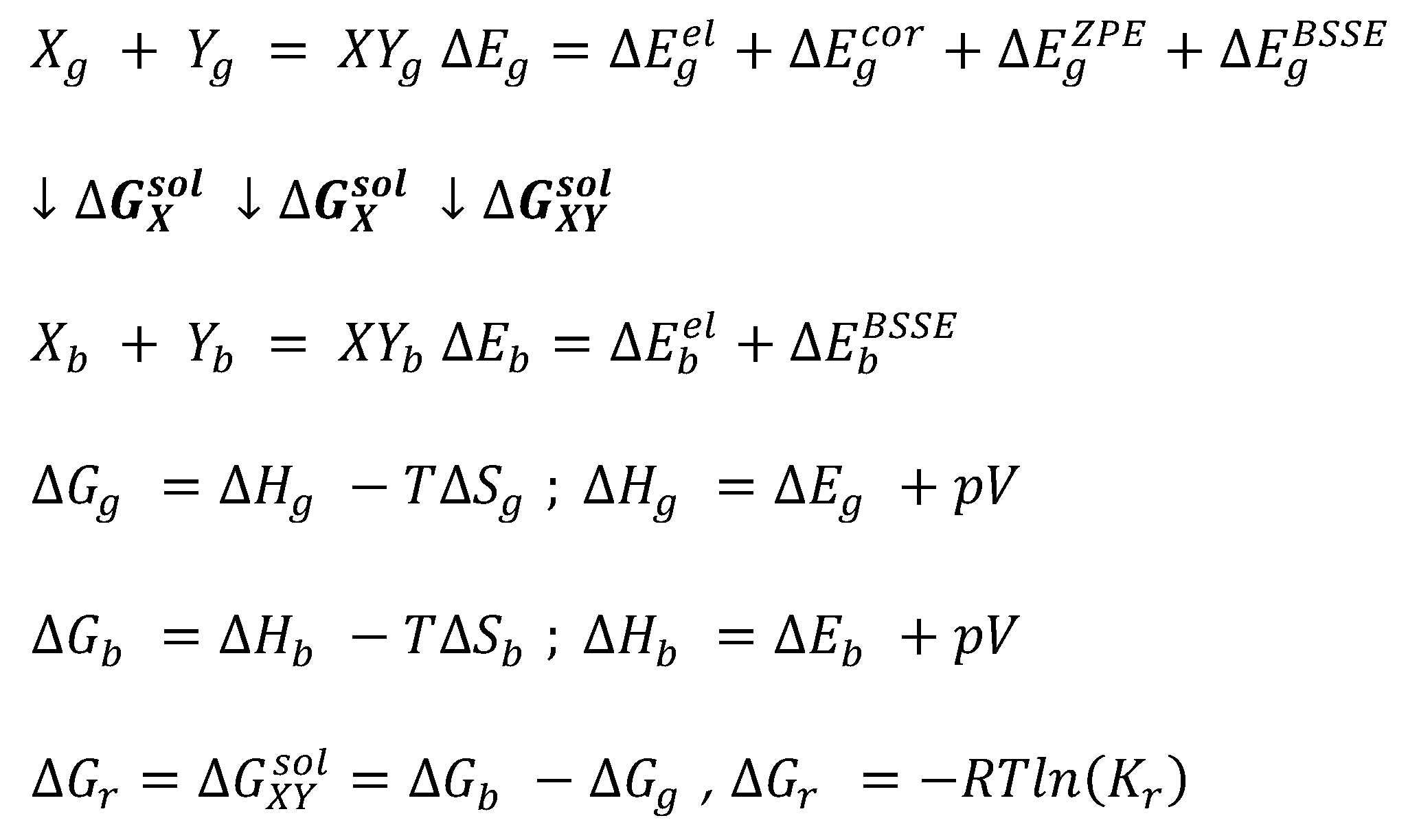
Figure ii. Solubility of caffeine, expressed as its mole fractions, in binary solvents comprising h2o and one of 5 studied aprotic proton acceptor solvents in varying compositions. On the abscissa, 10₂ ^* represents the mole fractions of organic solvent in solute-complimentary binary solutions.

Figure 2. Solubility of caffeine, expressed as its mole fractions, in binary solvents comprising water and 1 of five studied aprotic proton acceptor solvents in varying compositions. On the abscissa, 10_two ^* represents the mole fractions of organic solvent in solute-free binary solutions.

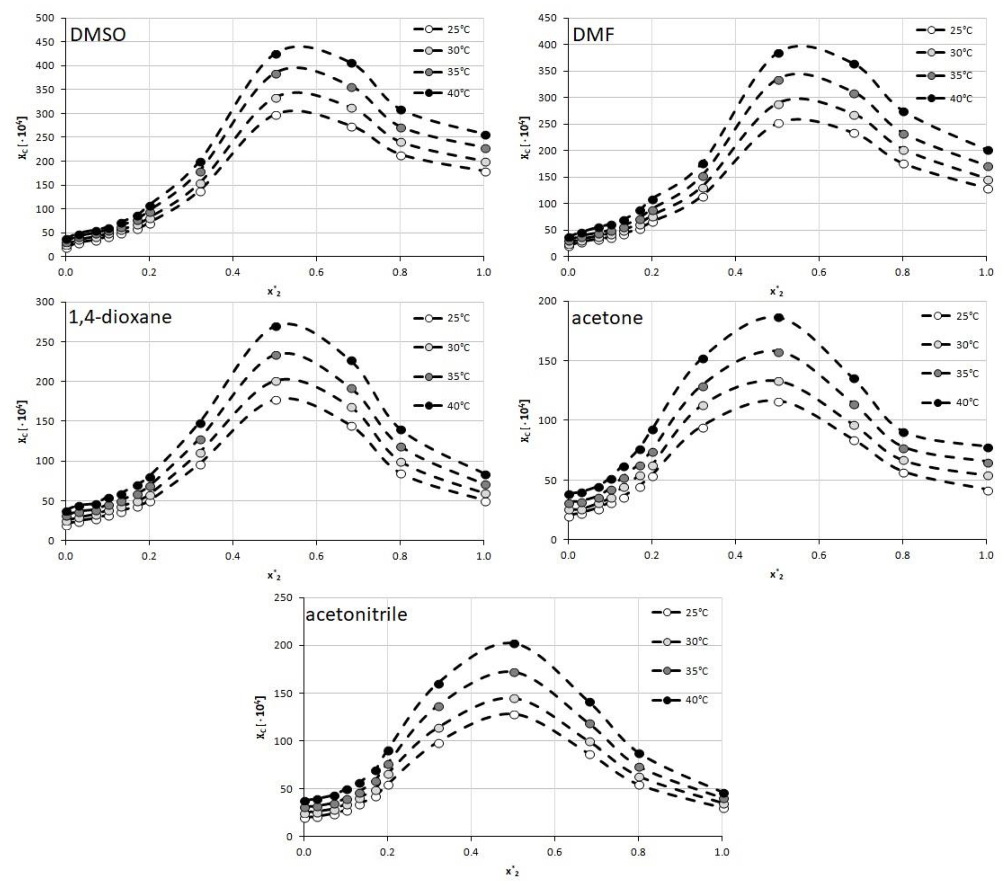
Figure three. Electrostatic molecule potential color-coded on density isosurface of caffeine representing the range from −0.05 eV to +0.05 eV. Colors signal electronegative (red) and electropositive (bluish) regions.

Effigy 3. Electrostatic molecule potential colour-coded on density isosurface of caffeine representing the range from −0.05 eV to +0.05 eV. Colors indicate electronegative (red) and electropositive (blue) regions.

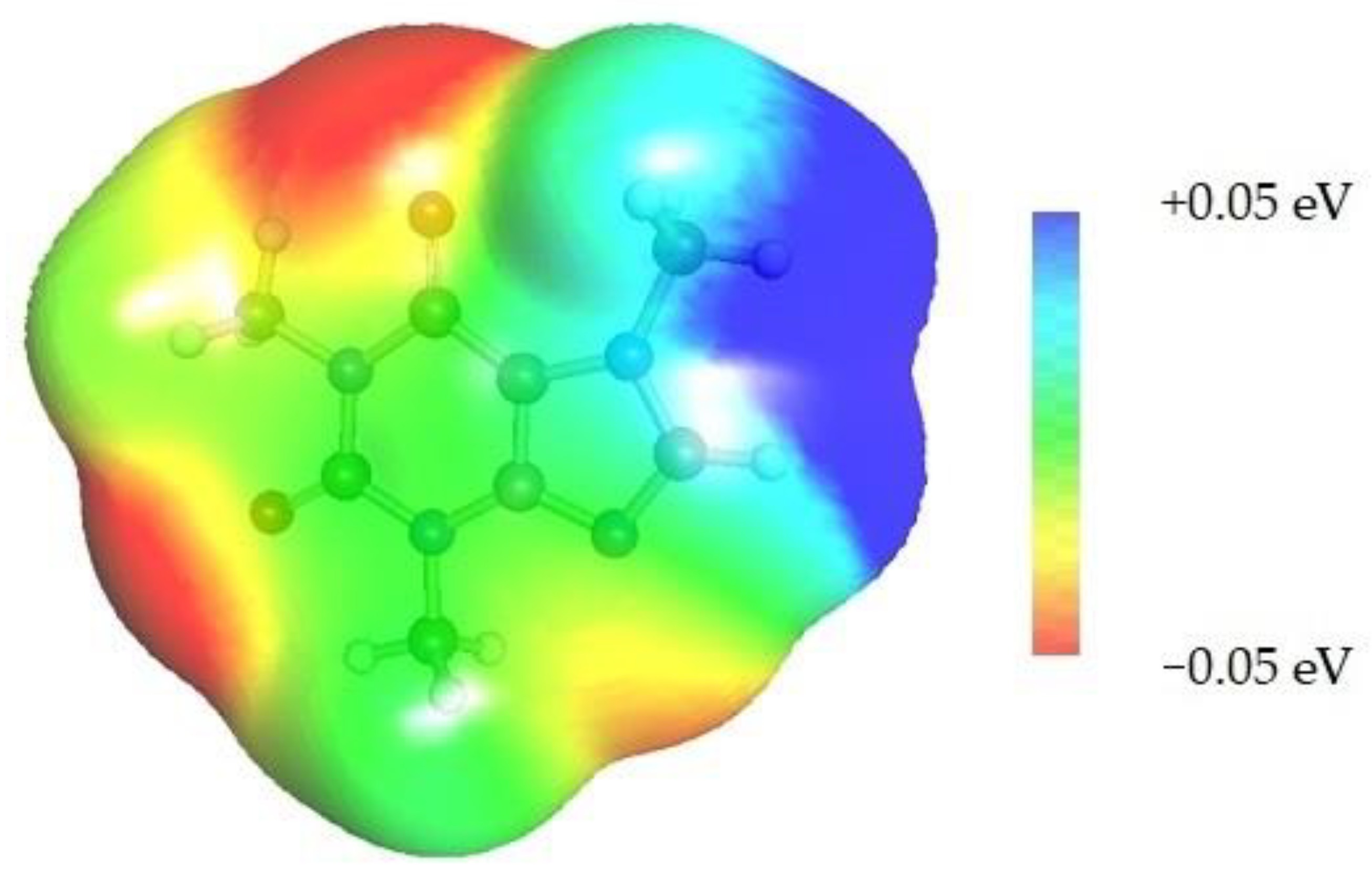
Figure four. The correlations between the experimental caffeine solubility in binary water-organic mixtures at 25 °C and the solute–solute (AA) affinities, solute–solvent (AB = AB1 + AB2) affinities and total affinities including solvent–solvent interactions (AA + AB + BB), where A stands for caffeine, B1 denotes the organic solvent, B2 denotes h2o and BB = BB1 + BB2 + BB12.

Figure 4. The correlations between the experimental caffeine solubility in binary water-organic mixtures at 25 °C and the solute–solute (AA) affinities, solute–solvent (AB = AB1 + AB2) affinities and full affinities including solvent–solvent interactions (AA + AB + BB), where A stands for caffeine, B1 denotes the organic solvent, B2 denotes water and BB = BB1 + BB2 + BB12.

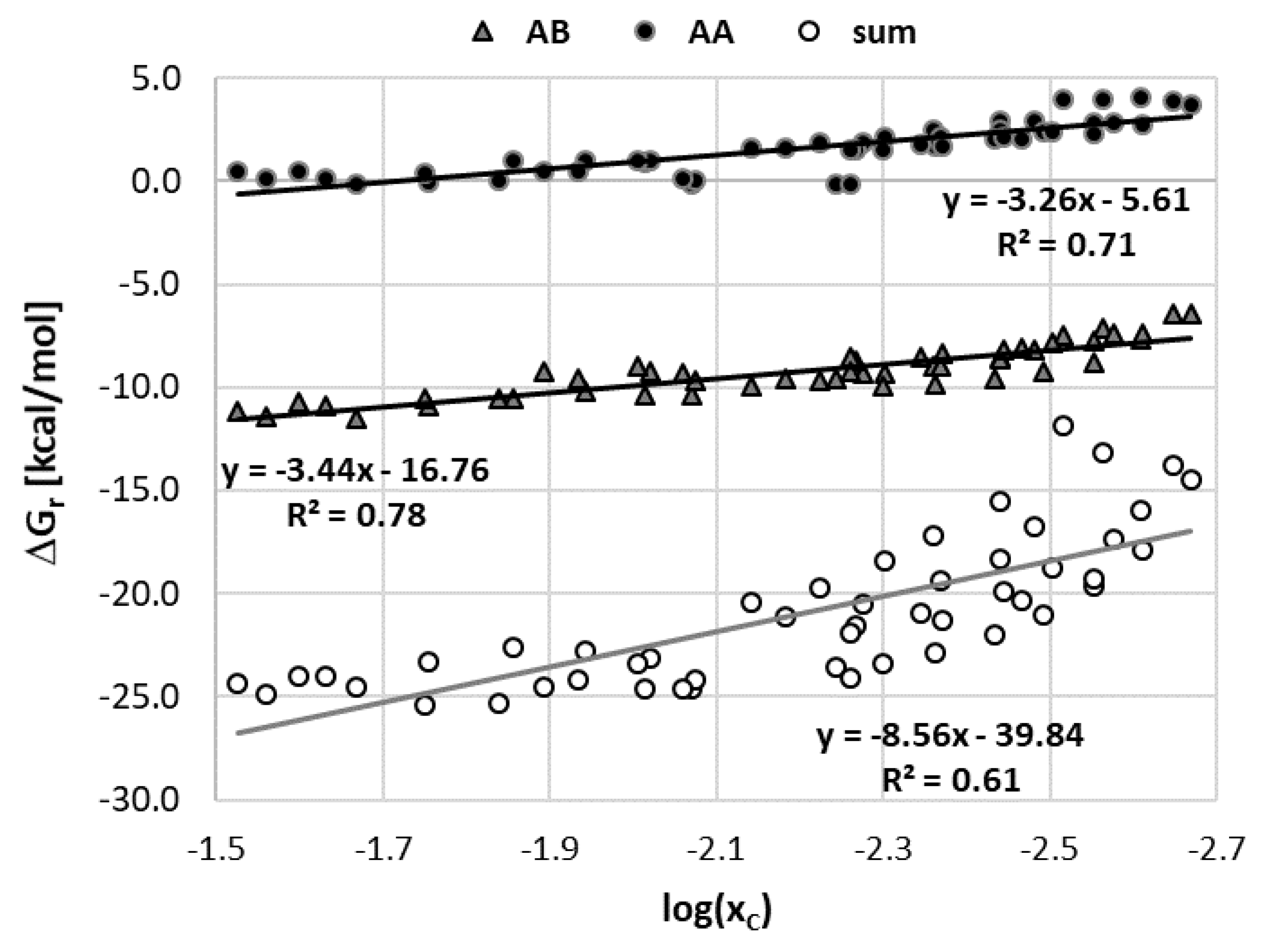
Figure five. The correlations betwixt the caffeine affinity computed at 25 °C and the composition of the binary solvent for the studied APAS.

Figure 5. The correlations between the caffeine affinity computed at 25 °C and the limerick of the binary solvent for the studied APAS.

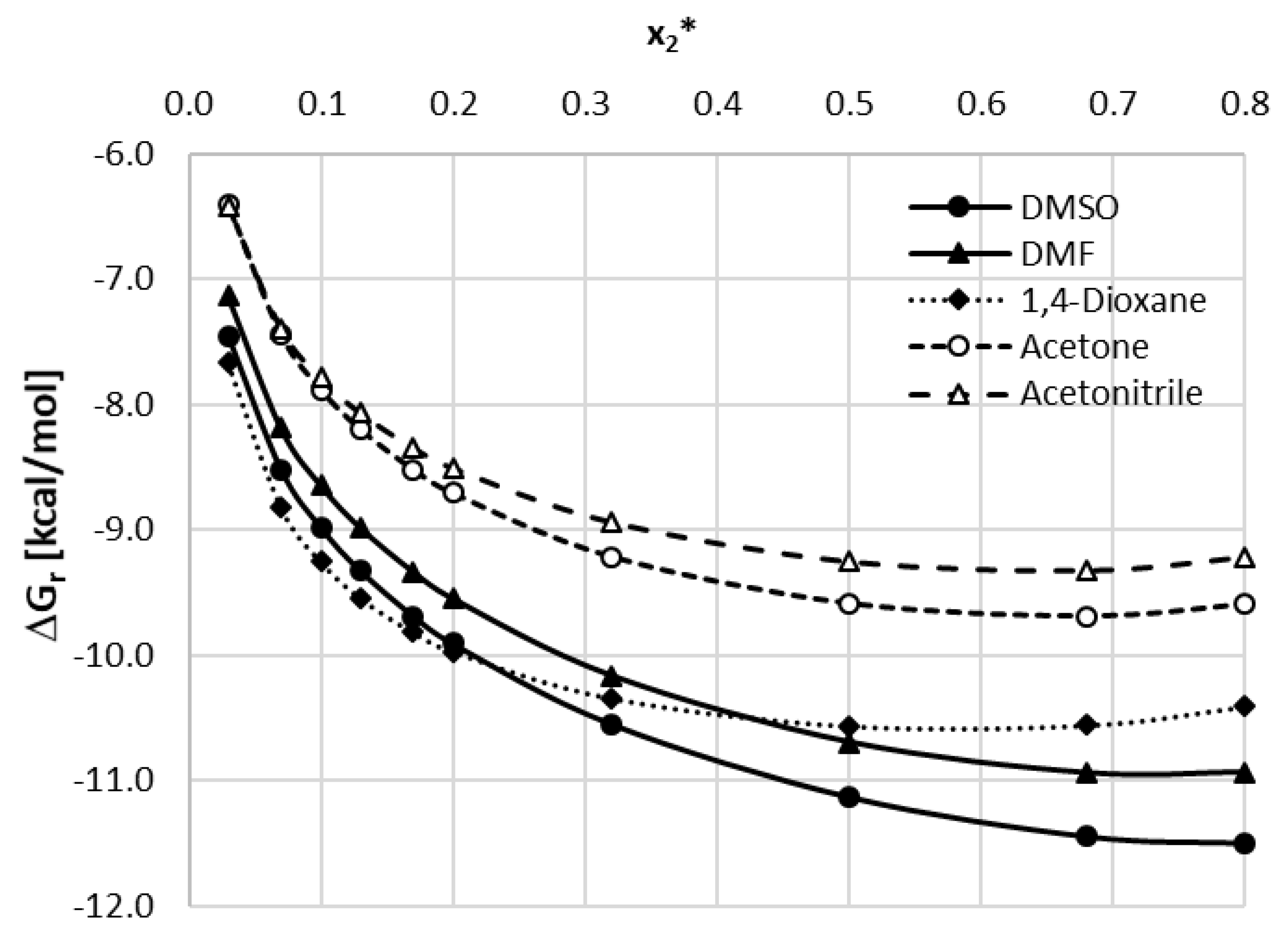
Figure six. Experimental solubility of caffeine, expressed as its mole fractions, in binary solvents comprising h2o and 4-formylmorpholine in varying compositions. On the abscissa, 10^* ₂ represents the mole fractions of organic solvent in solute-free binary solutions. Temperature was set to 25 °C and solubility values obtained in DMSO were shown for comparison.

Figure 6. Experimental solubility of caffeine, expressed as its mole fractions, in binary solvents comprising water and 4-formylmorpholine in varying compositions. On the abscissa, x^* ₂ represents the mole fractions of organic solvent in solute-free binary solutions. Temperature was set to 25 °C and solubility values obtained in DMSO were shown for comparison.

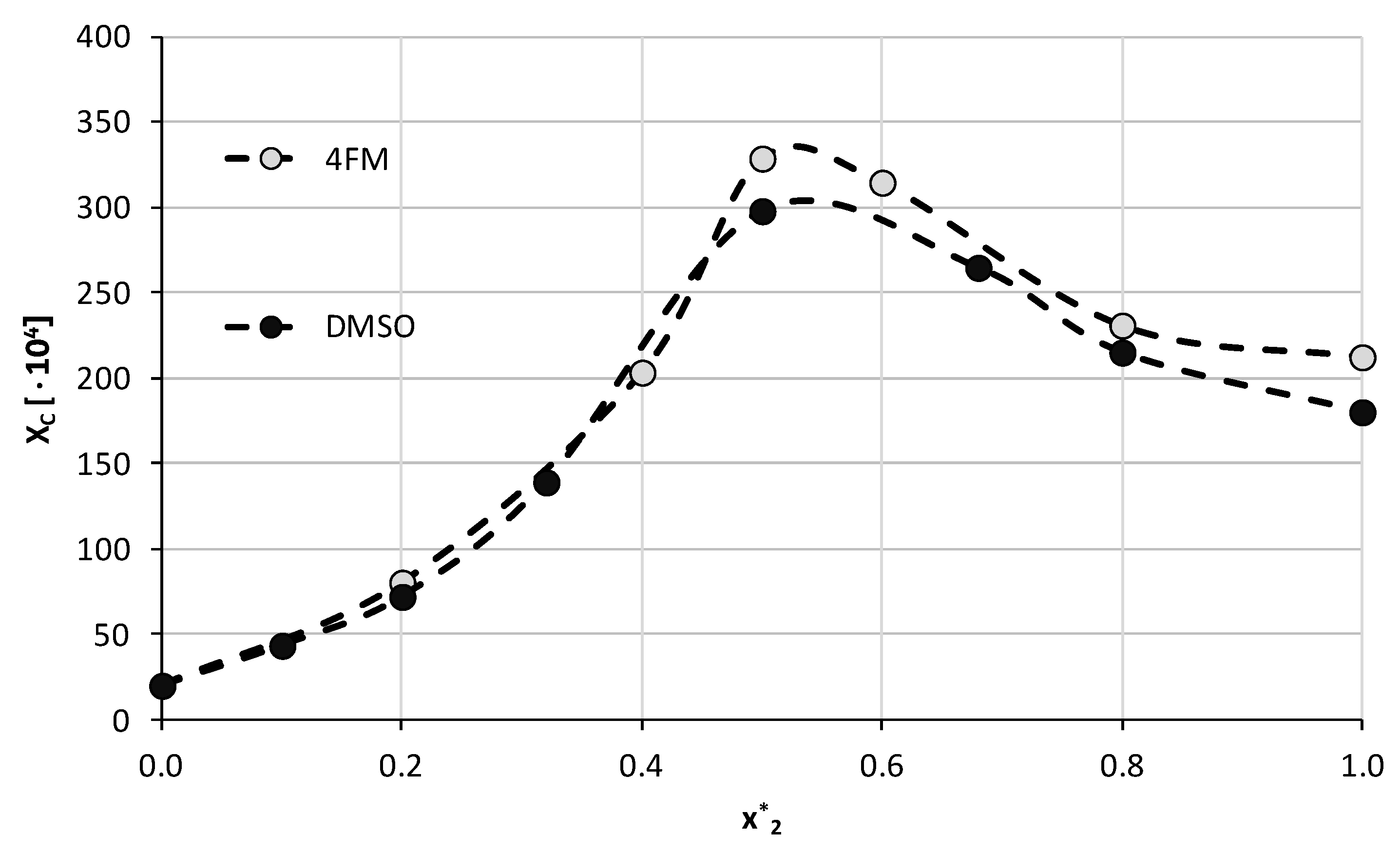
Table 1. Characteristics of the nigh stable bimolecular hetero-molecular complexes formed by caffeine in analyzed solutions. Primes in the geometry parameters announce atoms of solvent molecules. The values of Gibbs costless energy of reaction represent the concentration-independent quantity derived using activities at 25 °C.

Tabular array 2. Drove of environmental indices of mutual solvents used in this study and some morpholine derivatives.

Table 2. Collection of environmental indices of common solvents used in this study and some morpholine derivatives.

Solvent	CAS	EI	EI(PCOP=0)	TB [M]
DMSO	[67-68-five]	xi.68	0.26	462
DMF	[68-12-2]	2.16	ii.16	426
1,4-dioxane	[123-91-i]	five.26	0.97	375
acetone	[67-64-one]	one.27	0.66	329
acetonitrile	[75-05-viii]	1.88	ane.88	355
morpholine	[110-91-8]	2.95	two.95	401
iv-formylmorpholine	[4394-85-viii]	0.51	0.51	512
iv-methylmorpholine	[109-02-four]	1.93	ane.93	389
4-ethylmorpholine	[100-74-3]	ii.12	2.12	412

Table 3. Characteristics of the near stable bimolecular hetero-molecular complexes formed by caffeine with morpholine and its iii N-substituted analogs. Primes in the geometry parameters denote atoms of solvent molecules. The values of Gibbs gratuitous energy of reaction represent the concentration-contained quantity derived using activities at 25 °C.

Publisher'southward Notation: MDPI stays neutral with regard to jurisdictional claims in published maps and institutional affiliations.

© 2022 by the authors. Licensee MDPI, Basel, Switzerland. This article is an open admission article distributed under the terms and conditions of the Creative Commons Attribution (CC BY) license (https://creativecommons.org/licenses/past/4.0/).

We apply cookies on our website to ensure you lot get the best experience.
Read more about our cookies here.

We have just recently launched a new version of our website.
Help us to further improve by taking part in this short 5 infinitesimal survey here. here.

voorheesberfan.blogspot.com

Source: https://www.mdpi.com/1996-1944/15/7/2472/htm

Share this post